

The sampling methods presented in this article can be used at the reception, during production, or at the shipping of a company.
With regard to reception, we seek to validate the quality of a batch of materials or products received.
During production, we can use sampling plans to control batches of units we just produced. We could then repair the defective units during production.
On the shipping side, we validate the quality of our internal productions before shipping to our customers.
This ensures and controls our “external” quality. That is before the product leaves the company.
For more information on quality in general, check out our article on Business Quality!
Now, before continuing with the different sampling methodologies, let’s define what production batch sampling is.
In manufacturing, sampling consists of randomly selecting a small quantity of a batch of raw or finished products in order to estimate the quality of the entire batch. Sampling plans make it possible to estimate whether the quality of a lot meets the acceptable quality level (AQL) established by the company. In some cases, they also make it possible to assess the risk of accepting a batch that does not meet the AQL (company risk rated α) or of refusing a batch that meets the AQL (supplier’s risk-rated β).
The purpose of sampling is to verify that a lot is of the desired quality by inspecting as few parts as possible. This makes it possible to optimize inspection costs versus non-quality costs (internal and external).
Advantages and Disadvantages of Sampling Plans?
Advantages :
- Savings on inspection costs
- Reduction of non-quality costs
- Reduction of inspection errors
Disadvantages :
- Risk of accepting a poor quality lot or refusing a good quality lot (with an acceptable AQL)
- Less information available
- Requires planning, documentation, and training
Simple Sampling Plan
A sampling inspection plan consists of taking a sample of a given size from a lot and then inspecting characteristics in order to classify the units as conforming or non-conforming. Then, based on the results, a decision is made whether or not the batch is acceptable based on an agreed AQL.
The purpose of a sampling plan is therefore to Accept or Reject a lot. This is not to assess quality. It is an audit tool.
A simple sampling plan is defined by the sample size and the acceptability criterion. In a simple plan, only one sample is analyzed per batch.
Sampling Plan Terminology
- N = Batch size
- n = Sample size
- c = Acceptability criteria
- d = Number of defectives observed
Efficiency Curve
There are operating characteristic curves to measure the performance of a sampling plan. These curves show the probability that a batch with a certain proportion of defects will be accepted or refused.
The number of defectives in a random sample of size (n) follows a binomial statistical distribution with parameters n and p (proportion of defectives in the lot).
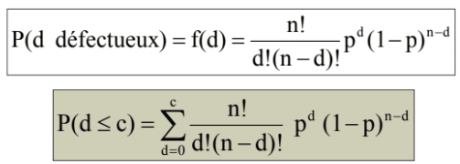
Where P( d défectueux) = P (d defective).
Here is an example of a curve for a plan n = 89 and c = 2.
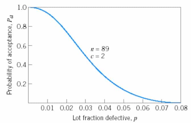
With this curve, we get the following acceptance probabilities:
| Proportion of defective (p) | Probability of acceptance |
| 0,005 | 0,9837 |
| 0,010 | 0,9397 |
| 0,020 | 0,7366 |
| 0,030 | 0,4985 |
| 0,040 | 0,3042 |
| 0,050 | 0,1721 |
| 0,060 | 0,0919 |
| 0,070 | 0,0468 |
| 0,080 | 0,0230 |
| 0,090 | 0,0109 |
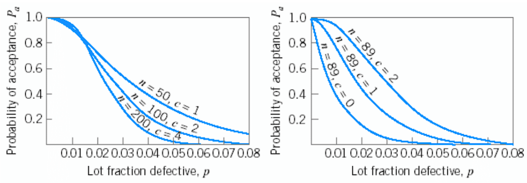
Effect of n and c on efficiency curves
Here are the effects of parameters n and c on the efficiency curves. The images are taken from chapter 15 of (Montgomery, 2013).
Designing a Simple Sampling Plan
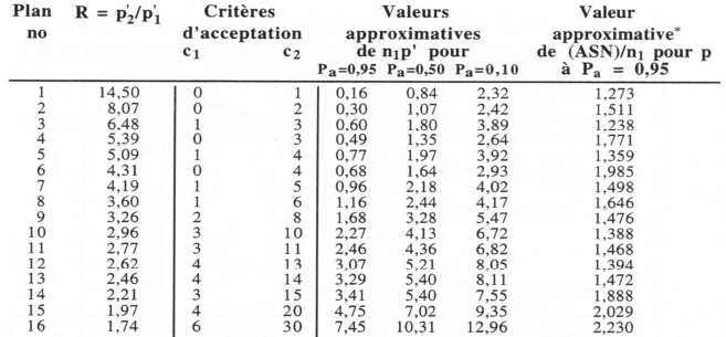
To design a simple plan, there are several methods. Here, we present Cameron’s method.
- Calculate the LTPD/AQL ratio. LTPD means Lot Tolerance Percent Defective
- Locate the value p2/p1 corresponding to the values α et β and look in Cameron’s table for the lower or equal value obtained in step 1 (LTPD/NQA). Take note of the value of criterion c.
- The size of the samples to be inspected per lot corresponds to np1/AQL
Where α = Probability of rejecting a lot of acceptable quality according to the AQL and β = Probability of accepting a lot of unacceptable quality according to the AQL
Simple Sampling Plan Example
Let’s take a lot tolerance percent Defective (LTPD) of 3% and an acceptable quality level (AQL) of 1.5%. The risks α and β determined are 5% each.
Then, LTPD/AQL = 0.030 / 0.015 = 2
In the Cameron table (which can be found on the internet), we find the value that is less than or equal to 2,000.
| Example of Cameron’s Table | ||
| c | α et β = 5% | np1 |
| 0 | 58,404 | 0,052 |
| 1 | 13,349 | 0,355 |
| 2 | 7,699 | 0,818 |
| … | … | … |
| 22 | 1,999 | 15,719 |
| 23 | 1,969 | 16,548 |
The sample size is therefore n = np1/NQA = 15.719 / 0.015 = 1047.933333 = 1048
Therefore, we obtain n = 1048 and c = 22.
Double Sampling Plan
Double sampling plans are defined by 4 parameters:
- n1 = Size of the first sample inspected
- c1 = Acceptance criteria for the first sample inspected
- n2 = Size of the second sample inspected
- c2 = Acceptance criteria for the second sample inspected
Double sampling plans require the inspection of two samples from a lot before making a decision on whether to accept or reject it.
Advantages and Disadvantages of Dual Plans
Advantages :
- Reduction in the number of inspections (batch is accepted or refused after the first sampling which is smaller than the ones from simple sampling plans)
- Reduced inspection cost
- Give the batch a second chance (++ for suppliers)
Disadvantages :
- There are some cases where the number of inspections becomes higher (therefore, the costs too)
- Higher risk of error (more complex at the administrative level)
Functioning of Double Sampling Plans – Example

Where d1 and d2 represent the number of defects identified in samples 1 and 2.
Designing of a Double Sampling Plan
To create a double sampling plan, you must follow the operation illustrated in the previous example and use a sampling table.
For example, one can use the tables of the Army Chemical Center or that of Schilling Johnson. We find tables where n1 = n2 and n2 = 2n1.
Table n2 = 2n1 – Army Chemical Center
Source : (Chemical Corps Engineering Agency, 1953)
Table n1 = n2 Schilling and Johnson for Simple and Double Sampling Plan
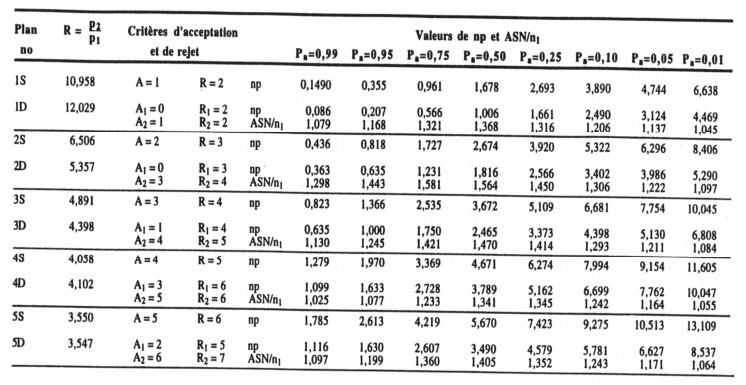
Whether it is the table of the Army Chemical Center or Schilling and Johnson, we find the acronym ASN (Average Sample Number).
ASN = n1 + n2 (1 – PI)
Multiple and Progressive Sampling Plans
Multiple Plans
Multiple plans require more than two samples to decide whether or not to accept the inspected lot. The sample required at each stage is smaller than for single or double plans.
| Cumulative sample size | Acceptance Criteria | Rejection Criteria |
| 20 | 0 | 3 |
| 40 | 1 | 4 |
| 60 | 3 | 6 |
| 80 | 5 | 7 |
| 100 | 8 | 9 |
Progressive Sampling Plans
For the progressive plans, the decision to accept, refuse or continue sampling is made after the analysis of each unit sample.
Advantages :
- Fewer parts to be inspected compared to an equivalent simple sampling plan (40 to 60% less)
- Batches of very good or very poor quality are processed very quickly
- Useful in the case of destructive testing or when inspection costs are high
Disadvantages :
- For batches between the NQA and the LTPD, a lot of units must be sampled (grey area)
- The number of units to be checked is undetermined (difficult to predict in advance)
- Complex. Requires proper training
Military Sampling Plan
Military tables were developed during the Second World War. Since the 1950s, they have been revised on 4 occasions.
Among the military tables, the MIL-STD 105E tables are the most used. It is therefore these that are presented in this section of the text.
MIL-STD 105E military tables allow 3 types of sampling. Single, Double, and Multiple Sampling.
For each type, there is a normal, reinforced, and reduced control. These will be explained a little later in the article.
Here are some features of the MIL-STD 105E tables:
- They are based on the acceptable quality level (AQL)
- The AQL is set by the company or in contracts with its suppliers and customers
- The size of the samples inspected is determined by the size of the lot and by the level of inspection chosen (I, II or III).
- There are special inspection levels noted S-1, S-2, S-3, and S-4.
Inspection Level:
The general inspection levels are levels I (less protection), II (normal protection), and III (more protection).
As for special inspection levels, they are used when:
- The samples used are very small
- The risk is greater but tolerated
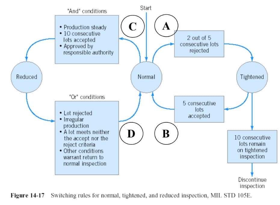
MIL-STD 105E Change Rule
The next figure is a reproduction of figure number 14-17 from the book “Introduction to statistical quality control” (Montgomery, 2013).
Procedures for Military Sampling (MIL-STD 105E)
- Determine the acceptable quality level (AQL)
- Choose the inspection level (I, II, III, S-1, S-2, S-3 or S-4)
- Determine the size of the batch received
- Determine the code letter (See Military table – next section)
- Identify appropriate tables for Normal, Reduced, and Enhanced control.
Example of Military Sampling (MIL-STD 105E)
A company wishes to place a simple plane in normal control (II). The lot size received is 5000 units and the AQL is 0.25%.
MIL-STD 105E Military Table:
| Special Inspection | General inspection | ||||||
| Batch size | S-1 | S-2 | S-3 | S-4 | I | II | III |
| 2-8 | A | A | A | A | A | A | B |
| 9-15 | A | A | A | A | A | B | C |
| 16-25 | A | A | B | B | B | C | D |
| 26-50 | A | B | B | C | C | D | E |
| 51-90 | B | B | C | C | C | E | F |
| 91-150 | B | B | C | D | D | F | G |
| 151-280 | B | C | D | E | E | G | H |
| 281-500 | B | C | D | E | F | H | J |
| 501-1201 | C | C | E | F | G | J | K |
| 1201-3200 | C | D | E | G | H | K | L |
| 3201-10 000 | C | D | F | G | J | L | M |
| 10 000-35 000 | C | D | F | H | K | M | N |
| 35 001-150 000 | D | E | G | J | L | N | P |
| 150 001-500 000 | D | E | G | J | M | P | Q |
| 500 001 + | D | E | H | K | N | Q | R |
Simple Sampling Plan – Normal inspection :
Image from (Montgomery, 2013)
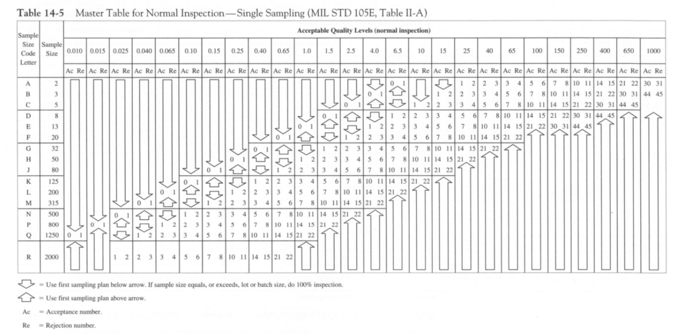
The company must therefore inspect 200 units per batch and the acceptability criterion (c) is 1 unit. That is to say, to be accepted, a batch must contain a maximum of 1 defective unit in the sample analyzed.
For the other tables, the principle is the same. We look for the letter corresponding to the plan and the required control, then we use the sampling table to determine the size of the samples to be inspected, then the acceptability criterion.
In the table, the rejection criterion “re” corresponds to the acceptability criterion + 1 unit. If a maximum of 1 defective unit is accepted, then the rejection criterion is 2 or more units.
Of course, you have to follow the rules of changes mentioned above to make sure you use the right tables. This will ensure the effectiveness of these sampling plans.
Finally, we find acceptable quality levels in percentage (0.01 to 10%), than in defects per 100 units (15 to 1000). Therefore, PPM (part per million) cannot be used with this type of plan (MIL-STD 105E).
Warning! It is not recommended to use the military tables without following the change rules!
Dodge and Romig Sampling Plan
Dodge and Romig sampling plans are used to inspect parts during manufacture. This type of plan allows 100% control and repair of defective parts (rectifying inspection) during production.
This avoids many additional non-value-added operations in the event of non-compliance. Despite everything, we must aim for zero defects and resolve the cause of the defects at the source.
Finally, the Dodge and Romig plans can be single or double and allow the use of PPM to target a quality rate. For example, an average acceptable quality limit (AQL) of 2% is equivalent to 20,000 defective parts per million. That is 2 x 1000,000 / 100.
Important element
For this type of plan, we use the limit level of tolerated quality (LTPD, “Lot Tolerance Percent Defective”) or the average quality limit after control (AOQL, “Average Outgoing Quality Limit”).
What is the difference between using LTPD or AOQL?
In the case of the limit level of tolerated quality (LTPD), it is used in the case of inspection of individual batches.
For a given LTPD, we seek to “minimize the long-term average controlled quantity and [the] average percentage of nonconforming units in the specific process (p)”(translated). (Baril, 2016)
On the side of the average quality limit after control (AOQL), it is used to inspect groups of batches with variable quality.
The goal is to “minimize the average long-term controlled quantity for a given AOQL and [the] average percentage of nonconforming units in the specific process (p). (translated) (Baril, 2016).
There are Dodge and Romig tables for single with AOQL, single with LTPD, double with AOQL, and double with LTPD plans. These are easily found here and there on the internet. You just have to make sure to choose the right tables according to the desired sampling plan.
Sample Simple Dodge and Romig Sampling Plan
A company wants to inspect electronic components on its assembly line. The batches are 15,000 units in size and the process has an average quality of 1.5% nonconforming units. The average quality limit after inspection (AOQL) is 3%.
The company uses the Dodge and Romig table for a simple sampling plan with AOQL = 3%. The table is shown below.
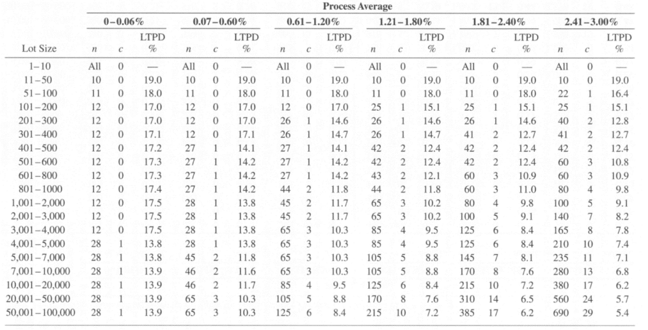
By consulting the table, the quality inspector of the company determines that he must inspect 125 units per batch and the acceptability criterion (c) is 6 non-compliant units. In this way, we ensure that we maintain statistical control of our process.
By making improvements and aiming for 0 defects, we want to try to minimize the “Process Average” or the average non-quality rate of our process.
Conclusion
In conclusion, sampling plans make it possible to accept or reject batches of raw materials, work in progress, or finished products.
There are different methods depending on the needs of the company and each methodology has its advantages and disadvantages.
The purpose of this article is to bring together a great source of information on sampling plans in order to answer all possible questions a reader may have regarding sampling.
In the article, single, double, multiple, and progressive sampling plans have been discussed.
Finally, tables and sampling plans were explained through some examples.
Reference :
Baril, C., (2016), Plan d’échantillonnage Simple Données d’attribut, pdf. Cours de Système d’assurance Qualité. UQTR.
Baril, C., (2016), Plan d’échantillonnage Double Données d’attribut, pdf. Cours de Système d’assurance Qualité. UQTR.
Baril, C., (2016), Plan d’échantillonnage Progressif Données d’attribut, pdf. Cours de Système d’assurance Qualité. UQTR.
Baril, C., (2016), Plan d’échantillonnage MIL STD 105E et ISO 2859 Données d’attribut, pdf. Cours de Système d’assurance Qualité. UQTR.
Baril, C., (2016), Plan d’échantillonnage Dodge et Romig Données d’attribut, pdf. Cours de Système d’assurance Qualité. UQTR.
Chemical Corps Engineering Agency, 1953. Manual No.2 : Master Sampling Plan for Single, Duplicate, Double and Multiple Sampling.
Montgomery, D., (2013), Introduction to statistical quality control, John Wiley & Sons.