Sales Forecast Excel: Complete Guide and Free Template!

 

Like you, we’ve done our research to find sales forecast information and tools. We couldn’t find anything significant, so we decided to compile this article to the best of our knowledge and expertise.

At the same time, we offer you a free Excel tool to make your forecasts!

Sales forecasting allows you to predict the future sales of a company. With the right method and depending on business variability, some models can achieve accuracy in the 90-95% range! However, this is not always the case, but it generally offers a more accurate sales forecast than doing it on the corner of a table.

During our visit to an SME that manufactures trailer wiring, we developed a tool similar to the one offered in the article. The tool’s accuracy was so good (+- 92% on average) that the company’s accountant kept it to continue using it.

Sales forecasts have several uses which are explored throughout the article. For example, budgeting, optimizing inventory management, etc.

 

 

What is a Sales Forecast?

 

The purpose of a sales forecast is to estimate a company’s future sales, in dollars or units, with the aim of :

• Plan the overall strategy of the company
• Optimize the allocation of internal resources
• Determine the cash needs of the business
• Determine when to increase production capacity
• Optimize inventory management
• Improve production planning and scheduling

More generally, one could define sales forecasting as a “function to estimate future demand that one establishes either mathematically (historical data), intuitively (market knowledge), or both. (Drolet, Robitaille & Désilets, 2016).

There are different software available to calculate and estimate a company’s sales forecasts. You can also use Excel and program the various forecast models to obtain very good results without having to pay a penny!

In this text, an Excel file with the most popular sales forecasting methods is offered to readers! Each of the methods is presented and the file is explained to facilitate its use. The performance indicators of the forecasting methods are also presented and can be found in the proposed tool. Here is an example of this file completely free!

 

 

Sales Forecast and Time Horizon

 

Long term :

Long-term forecasts have a horizon of 2 to 5 years. They are used in the strategic planning of the company.

The analysis of this type of forecast makes it possible, among other things, to plan plant expansions, increase production capacity, purchase new equipment or technologies, personnel needs, etc.

Conversely, it can make it possible to establish recovery strategies in the event that sales are down.

 

Middle term :

In the medium term, sales forecasts are established over 1 to 2 years. This time around, the purpose of their analysis is to determine the “operating budget of the business and some capital budget expenditures”.

 

Short term :

Finally, short-term forecasts are made over 1 year or less. They need to be precise and are used to carry out the planning of production activities, scheduling, inventory management, etc.

The analysis of short-term forecasts is essential for evaluating and optimizing a company’s operations. This can lead to significant savings. However, poor analysis can also lead to significant losses, hence the importance of data accuracy.

A good analysis and a good forecasting model can reduce the costs of storage, handling, logistics, etc.

 

Sales Forecasting Challenges

 

There are various reasons that make it difficult to accurately forecast the future demand of a business. The main reasons are:

• New products on the market
• Removal of an existing product
• Competitor promotions
• Price variation (raw material, energy, etc.)
• Economic context
• New technologies

These challenges can fluctuate company sales and make forecasting models less accurate. This means that we can overestimate or underestimate future demand.

If we overestimate demand, we risk underutilizing our staff and storing a lot of products. This will increase storage costs and tie up cash on inventory that is “sleeping” on the floor.

Conversely, by underestimating market demand, there is a risk of having to resort to overtime to subcontracting (and therefore increasing the unit production cost), running out of stocks (raw material), and delivering late. among customers (loss of trust with the customer).

 

 

Role of Sales Forecasts in Business Budgeting

 

A company’s budgeting plays a fundamental role in its ability to maintain sound cash management.

Before even getting into the concepts of budgeting, it is essential to understand the nuance between profitability and liquidity.

Profitability is the company’s ability to make a profit. By adding up all the income and subtracting this sum from all the expenses, we obtain the profit (also called net profit) of a company for the period studied. When managers evaluate a project, they ensure that the project will be profitable. Nevertheless, the project may well be potentially profitable, but the company must also be able to support this project financially. This is where liquidity management comes into play.

The liquidity of the company must be assessed regularly. Managers must ensure that they have sufficient funds to meet their obligations. Examples of obligations are the payment of a loan taken out with a financial institution, the payment of suppliers on time, the payment of a financial lease, the payment of employee salaries, the payment of subcontractors, etc. In other words, cash management comes down to being able to make a payment at the agreed time.

That being said, budgeting for a business is all about cash management.

 

What is a Business Budget?

 

Budgeting allows you to predict future cash inflows and outflows. This way, managers know if they will be able to make their payments on time. In the context where managers notice that there will be a lack of liquidity at a specific time, they will have to find sources of external financing. In other words, they will have to make up for the shortfall by borrowing, investing their personal funds, finding other investors, delaying their payments, etc. Generally, companies have a line of credit already authorized to offset deficits, but this is limited.

The purpose of budgeting is to forecast cash inflows and outflows as accurately as possible. Obviously, the variability of forecasts leads managers to make erroneous decisions. It is therefore essential to ensure that the source of the forecasts is valid, otherwise, the entire budgeting of the company is biased.

The source of all business budgeting is the sales forecast.

 

Importance of Sales Forecasting for the Corporate Budget

 

You’ve probably heard the expression “Garbage in, Garbage out”. The main input of budgeting is revenue forecasting. When sales are forecasted, this forecast acts as the starting point for establishing the sales budget.

This is the first budget to be made from a set of budgets called the master budget. The objective behind the realization of the master budget is to forecast all the inflows and outflows of funds. This will make it possible to achieve the cash budget.

The cash budget is the summary that allows the company to see which periods of a year will be in surplus or in a deficit of liquidity. This budget is then used to establish the projected financial statements of the company.

Here is a table with some links to each budget a Business could need!

 

Manufacturing Company	Commercial Enterprise	All Companies
Production Budget	Inventory Budget	Sales Budget
Raw Materials Budget	Goods Purchase Budget	Selling and Administrative Expense Budget
Direct Labor Budget		Cash Budget
Business Expenses Budget
Inventory Budget

 

In summary, knowing that the sales forecast has a major impact on the entire budgeting of the company, it is crucial to give it a high degree of importance.

All the more, when we know that one of the most important financial problems of companies is the lack of liquidity, we must redouble our efforts and master the management of liquidity!

Now, how to effectively predict future sales? The next sections deal with sales forecasting methods and using the free Excel file to forecast your sales.

 

What are the Sales Forecasting Methods?

 

There are three types of forecasting methods depending on the company’s sales environment: stable, trending, or seasonal.

 

 

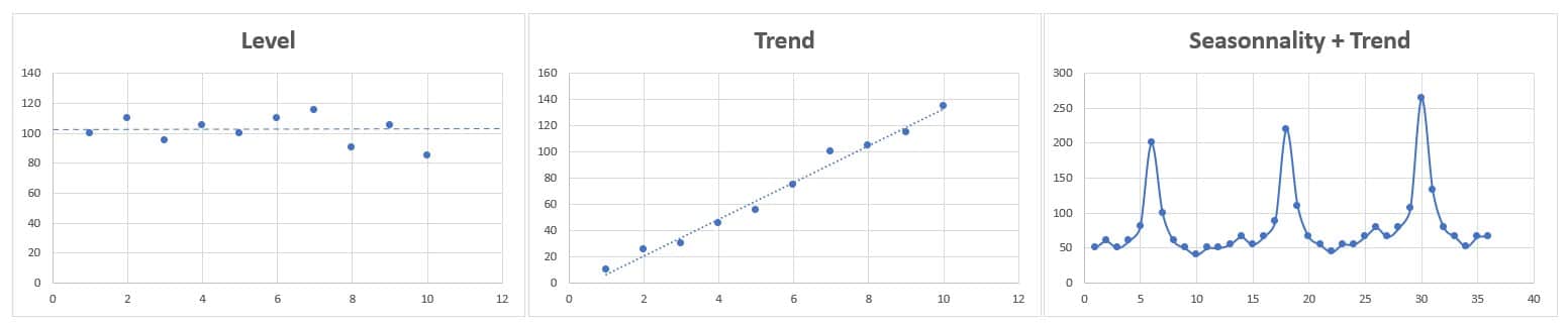
The methods, presented in this text, for companies that are stable, i.e. their sales follow a level or an average are:

• Naive forecasts
• Simple Arithmetic Means
• Simple Moving Averages*
• Weighted averages*
• Simple Exponential Smoothing*

*Methods available and automated in the free sales forecast template!

 

For businesses that are growing, or following a trend, the methods presented are:

• Simple Linear Regression*
• Multiple Linear Regression*
• Trend Analysis (Average Variation)*
• Double Moving Average*
• Simple Exponential Smoothing with trend component*
• Double Exponential Smoothing*

 

Finally, for businesses with seasonality, the methods are:

• Forecast using seasonal index (+linear regression)*
• Seasonal adjustment method
• Winters method

 

Sales Forecast Methods and Performance Indicators

 

Before continuing with the predictive methods in more detail, here are the main performance indicators to assess the accuracy of the tools.

In the Excel file, the indicators are used to determine at a glance which method is the most suitable (accurate) for you!

The different indicators are:

• The Error or Deviation
• The Bias or Mean Error
• Relative Absolute Error (RAE)
• Mean Absolute Deviation (MAD)*
• Mean Squared Error (MSE)*
• Root Mean Absolute Errors (RMSE)*
• Correlation Coefficient (R)*
• Coefficient of Determination (R2)*

*Indicator used in the Free sales forecast template

 

Error or Deviation

 

The error or deviation (E_i) is the difference between the actual sales R_i and the sales forecast P_i for a period “i”.

E(i) = R_i – P_i

 

Bias or Mean Error

 

The average bias or error represents the average of the errors (deviations) observed after a number of periods n.

The mean error indicates whether a method tends to give predictions above or below the mean.

Bias = ∑ i=1 to n (R_i – P_i / n)

 

Relative Absolute Error (RAE)

 

The absolute relative error represents the error as a percentage. RAE gives an indication of the accuracy of a method or establishes a confidence interval for making a prediction.

Precision: RAE(i) = |R_i – P_i| / R_i

Confidence Interval: RAE(i) = |R_i – P_i| / P_i

Where Ri: Actual sale for period i, Pi: Demand forecast i, and i: Period index

 

Mean Absolute Deviation (MAD)

 

The mean absolute deviation “considers the size rather than the direction of the forecast error. A low EMA indicates that the method used helps predict demand very well. (Drolet, Robitaille & Desilets, 2016)

MAD = ∑ i=1 to n (|R_i – P_i| / n)

 

Mean Squared Error (MSE)

 

The mean squared error squares for each of the forecast errors. In this way, the RMSE indicates whether a model provides more often than the other large forecast deviations.

RMSE = ∑ i=1 to n ((R_i – P_i)² / n)

 

Mean Absolute Relative Errors (MARE)

 

The mean of absolute relative errors is a good performance indicator for methods. It is used to determine whether a forecast model is accurate or not.

MARE = (∑ i=1 to n (R_i – P_i / n) / R_i) / n

 

Correlation Coefficient (R)

 

The correlation coefficient (R) “indicates the degree of relationship between a dependent variable and an independent variable. (Drolet, Robitaille & Desilets, 2016)

The closer R is to 1 (or -1) the stronger the relationship.

(-1 ≤ R ≤ 1)

R = (n∑xy – ∑x∑y) / √[n∑x²–(∑x)²][n∑y²–(∑y)²]

 

R =	Meaning
0,90 à 1,00 OU -0.90 à -1,00	Very Good Correlation
0,70 à 0,8999 OU -0,7 à -0,8999	Good Correlation
0,40 à 0,6999 OU -0,4 à -0,6999	Low to Medium Correlation
-0,3999 à 0,3999	Poor to No Correlation

 

Coefficient of Determination (R²)

 

The coefficient of determination (R²) “corresponds to the percentage of the variation of the dependent variable explained by the independent variable”. (Drolet, Robitaille & Desilets, 2016)

The closer the coefficient of determination is to 1, the more accurately one can predict the value of the dependent variable (y) based on the value of the independent variable (x).

In other words, the mathematical model relating x and y are exact when R² = 1. This method is used to determine model accuracy using linear or multiple regressions.

Finally, consider the following example. A determination coefficient R² = 0.9 is obtained. This indicates that 90% of the variation of variable Y is explained by the variation of variable X. The remaining 10% varies according to other unknown variables of the mathematical model.

 

 

Forecasting Methods Without Trend Or Seasonality – Sales Forecasting model

 

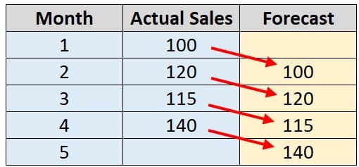
Naïve Forecasting sales

 

The naïve method is very simple, and inexpensive, but not very precise. For these reasons, we have decided not to include it in the Free Excel file.

This method consists of using the actual sale of period i-1 as the forecast for period i.

Example:

 

Simple Arithmetic Means

 

For this method, the average of past actual sales is used to determine the forecast for the next period. It is a low-cost, simple, but inaccurate method “in the context of dynamic demand.” This method requires keeping a certain amount of data.

This method is also not available in the Excel file, since the precision is often low.

It is possible to use this method for seasonal demands. In this case, the average of the periods of the past “seasons” is used. For example, for June 2022, we use the average sales of June 2018, 2019, 2020, and 2021.

Example:

 

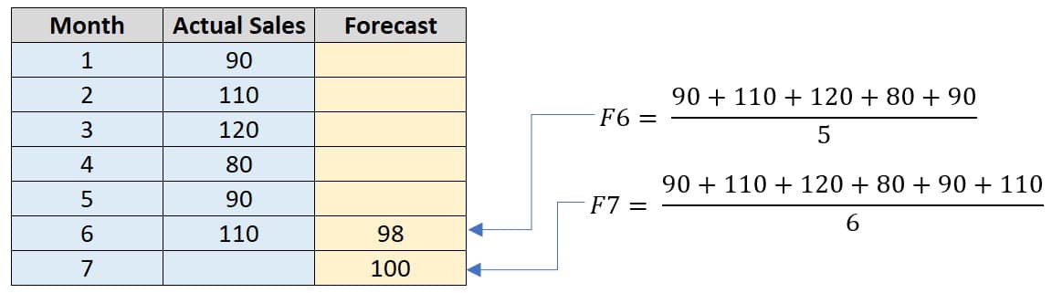
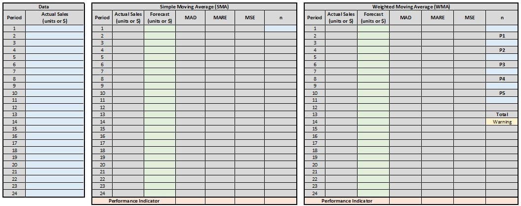
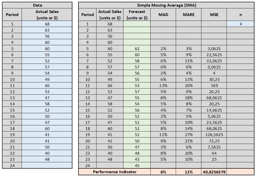
Simple Moving Average (SMA)

 

The simple moving average method is the first in the article that is available in the free sales forecast calculator.

It is a popular and easy-to-use method. This model should be used for sales without trends or seasonality. It allows you to calculate forecasts for a period in the future (you have to feed the model as you go to calculate the forecasts for each period).

The principle of the simple moving average is to use the average of actual sales for a number of previous periods for the purpose of forecasting sales for one period in the future.

Only a certain amount of data is used to calculate the average, i.e. the most recent. We always use the same number of data to calculate the SMA (we determine the number of data “n” before starting).

Concretely, the formula used to calculate the simple moving average is as follows:

P(t+1) = ∑ i=t to T (R_i) / n

Where n = number of data used to calculate the average, i = first period considered in the calculation of the SMA, and t = last period used in the calculation of the SMA.

Here is what this technique looks like when used with our free sales forecast templates

 

Simple Moving Average – Excel Tool

 

For all methods, the principle remains the same. Enter your data in the blue boxes and the forecasts, as well as the performance indicators, will be calculated automatically.

The forecasts are in the green boxes and the performance indicators are in the beige boxes. Some boxes have comments as a reminder. For example, what are performance indicator acronyms, and how to interpret them?

Finally, for the simple moving average, the file offers the possibility of using an “n” equal to 4, 5, or 6.

 

 

Weighted Moving Average (WMA)

 

The weighted moving average is similar to the simple moving average, but this time we give importance (weight) to each value used to calculate the average.

When using the simple moving average with say n = 4, each value equals 25% of the final result. The MMP makes it possible to modify this weighting, for example, to give more importance to more recent values.

The formula for calculating weighted moving averages is:

Mi = ∑ L=1 to n (a_L*X_i-L)

Where Mi = weighted moving average for period i, n = number of periods used for the calculation of MMP, Xi-L = actual sale for a previous period, and aL = weight or weight of security in the calculation of the average.

Note: The sum of aL must equal 1 (or 100%).

 

Weighted Moving Average – Excel Tool

 

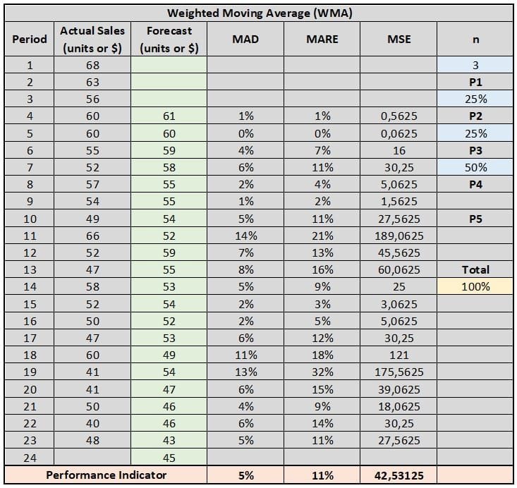
1. Begin by entering data into the “Data” table in blue.
2. Select the “n” that suits you at the top right of the table titled “Weighted Moving Average (WMA)”. You have the choice between n equal to 3, 4, or 5.
3. In boxes “P1” to “P5”, enter the weighting of each of the values. P1 is the weight of the oldest value and P5 is the most recent. Depending on whether you select “n” equal to 3, 4, or 5, you will need to fill in boxes “P1” to “P3”, “P4” or “P5”. The sum of the weights must be 100%. The “Total” box in yellow gives the sum of the weights. It will show a “Warning” if the sum of the weights is different from 100%.
4. The green boxes show the sales forecast for this model.
5. The beige “Indicator Performance” boxes show the accuracy of the method. They allow you to compare the different methods at a glance.

Note: By filling in the “Data” boxes, all methods in a tab will perform this calculation. For example, all sales forecast methods for demand without trend or seasonality will be calculated. You can choose the most accurate by consulting the performance indicators.

 

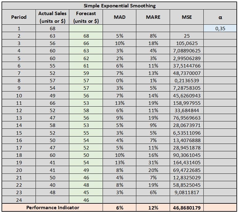
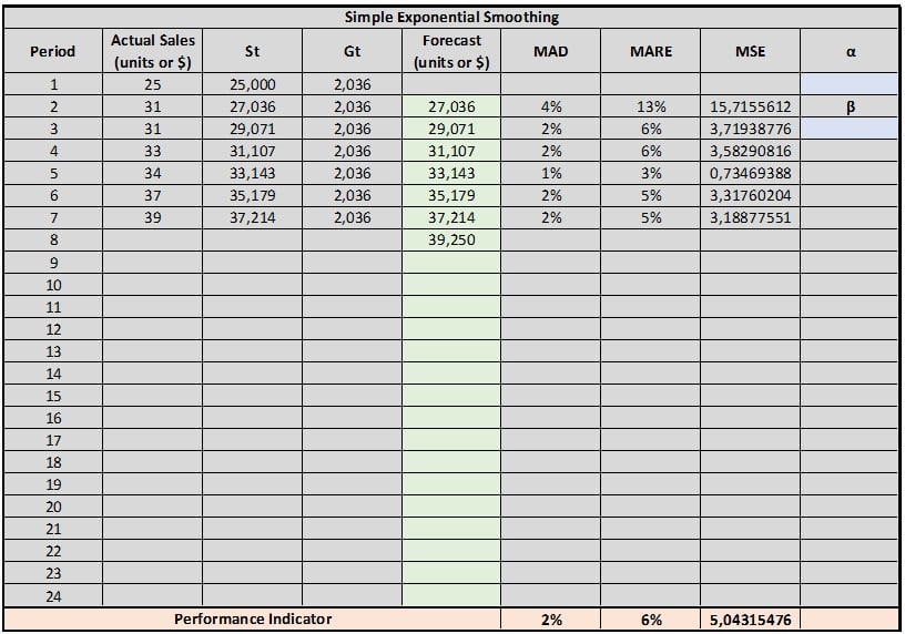
Simple Exponential Smoothing (SES)

 

Simple exponential smoothing is a simple method to use and often gives better results than a simple moving average. This method allows you to estimate sales for one period in the future at a time.

The principle of LES is “based on the fact that the current forecast matches the previous forecast adjusted somewhat”. To adjust the latter, a weighting factor α (usually between 0.1 and 0.3) and the difference between the last forecast and the actual sale are used.

For single exponential smoothing, the following formula is used:

S_T = α*X_T + (1 – α)*S_T-1

Where ST = estimated sales at time T, α = smoothing parameter, XT = demand at period T and ST-1 = estimated sales at period T-1.

The weighting factor α “determines the level of smoothing and the speed of reaction to the difference between forecast and actual demand. (Drolet, Robitaille & Désilets, 2016).

The more fluctuating the demand, the more a high α is needed to obtain an accurate model. Conversely, stable demand requires a smoothing parameter close to 0.

 

Simple Exponential Smoothing – Excel Tool

 

Forecast Methods With Trend – Sales Forecast

 

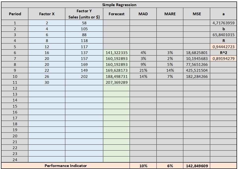
Simple Linear Regression

 

Simple linear regression establishes a linear relationship between two factors (variables). One of the variables is dependent (y) on the other (x, independent variable). The established relationship takes the following form:

Y = ax + b

The parameters “a” and “b” represent the slope of the linear line and the y-intercept, respectively. This method requires some historical data to establish an accurate linear relationship. To know the accuracy of this model, we use the coefficients of correlation “R” and determination “R²“.

There is a table showing the meaning of “R” based on its value in the section about performance indicators.

For the coefficient of determination, the closer the value of “R²” is to 1, the better the relationship between x and y. For example, an R2 = 0.9 indicates that 90% of the value of Y is explained by the variation of the independent variable x.

 

Simple Linear Regression – Excel Tool

 

Multiple Linear Regression

 

Multiple regression is, according to (Drolet, Robitaille & Désilets, 2016), “an extension of simple linear regression allowing several independent variables X to be taken into consideration in order to explain the behavior of a dependent variable Y.” independent variables X1, X2, …, Xn.

The multiple regression follows a mathematical function: Y = b0 + b1X1 + b2X2 + … + BnXn

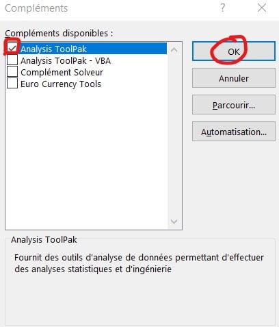
To access multiple regression on Excel, you must first install/add the Excel analysis utility. Here’s how to add it if you haven’t already:

 

Step1: Go to File

 

 

 

Step2: Click on “Options”, then add-in, and finally “Go to”

 

               

 

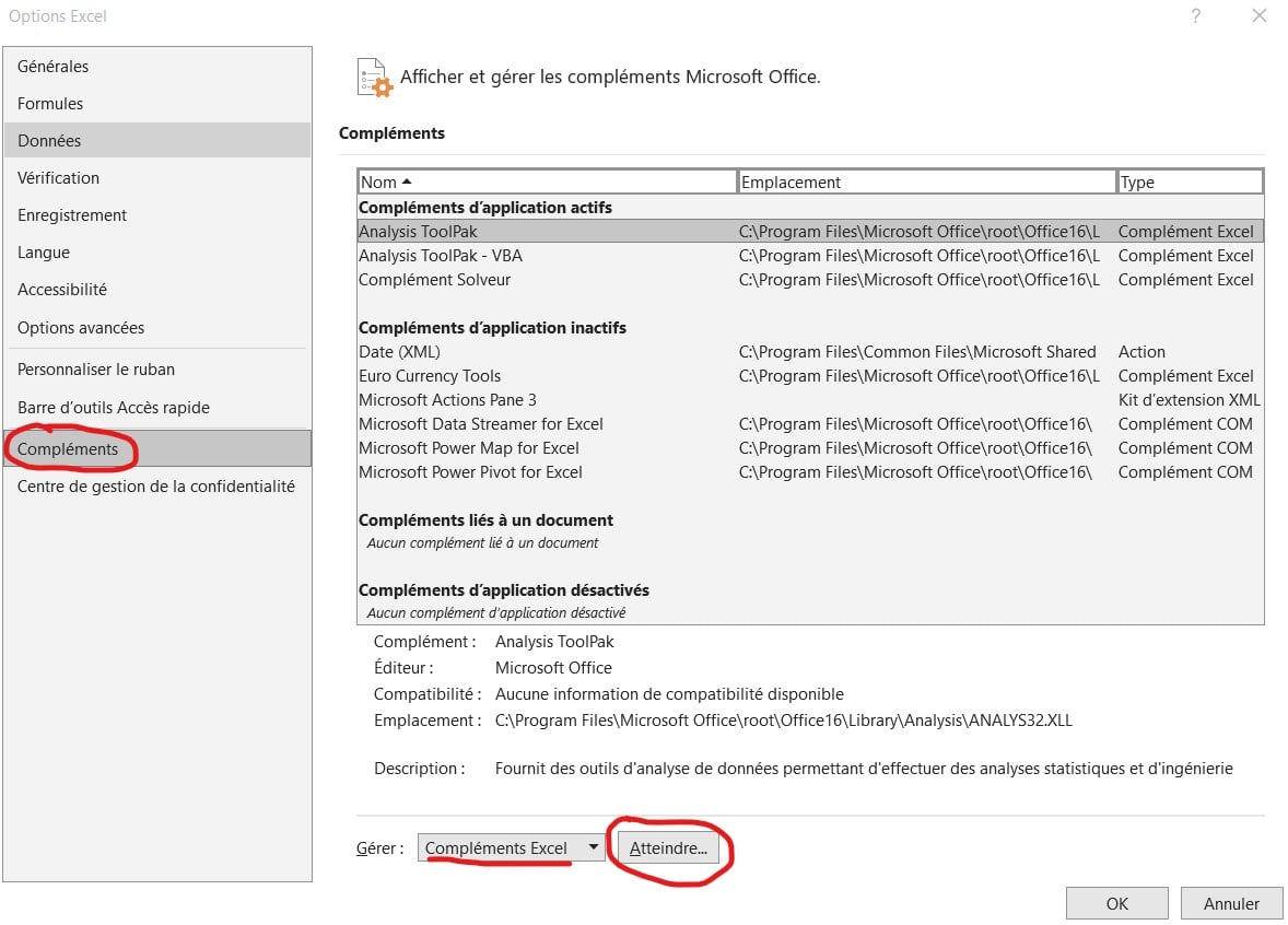
Step3: Select “Analysis Utility” or “Analysis Toolpack”

 

 

Multiple Linear Regression – Excel Tool

 

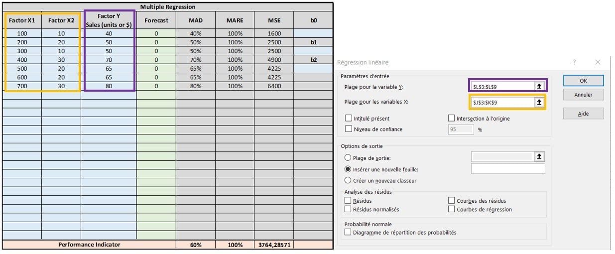
To use multiple regression with the file provided in the article, here’s how:

Step 1: Enter your data in the table titled “Multiple Regression”

 

 

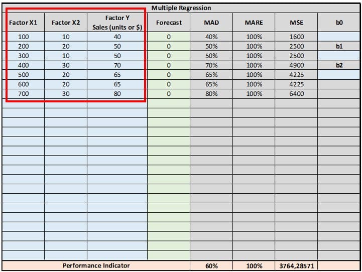
Step 2. Launch the analysis utility in the “data” tab and select linear regression

 

 

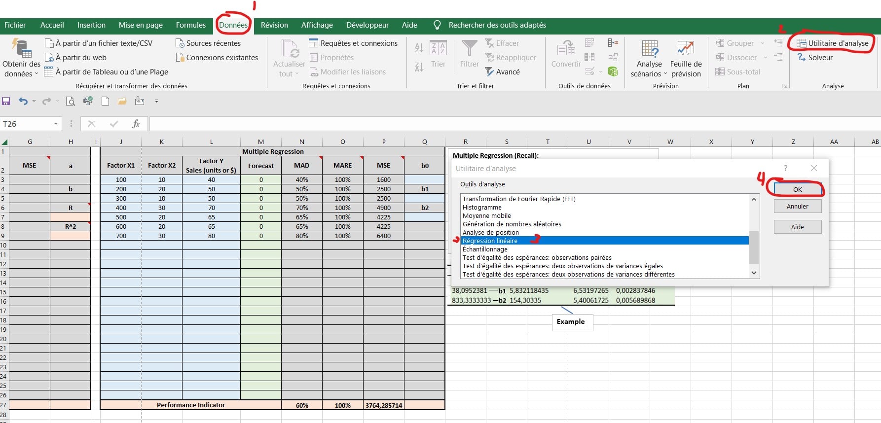
Step 3: Enter the dependent variables (“X1” and “X2”) and the independent variable in the places shown below.

 

 

Step 4: With the results obtained, we obtain the coefficients of determinations, the ordinate at the origin, and the slopes of the equation, as well as the Student statistics to verify that the independent variables do indeed have an effect on the independent variable (with a confidence level of 95%).

 

 

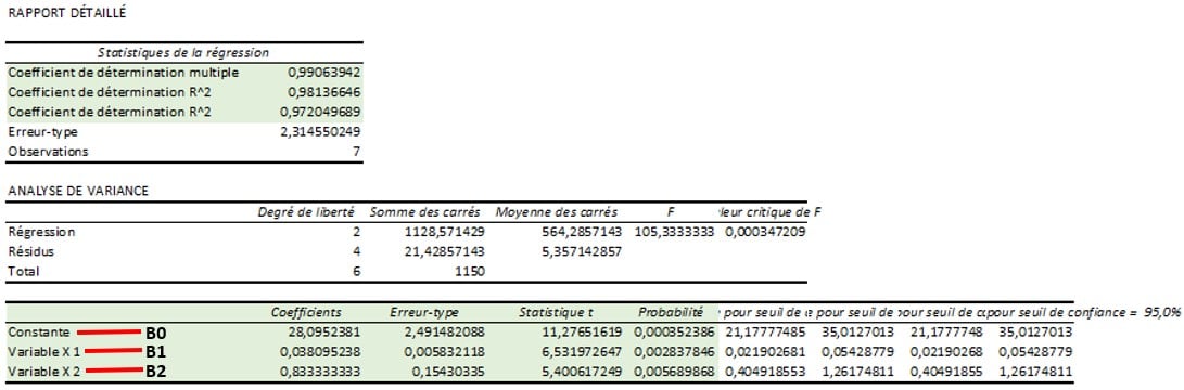
In this example, we see that the Student statistics give a probability of 0.002837 for “X1” and 0.005689 for “X2”. These probabilities are less than 0.05, so we can say that the independent variables have an effect on the dependent variable with a confidence level of 95%.

The multiple coefficients of determination of 0.9906… indicates that the model explains 99% of the variation of “Y”. Which is very good. (See the explanation for the coefficient of determination in the “Linear Regression” section as needed).

 

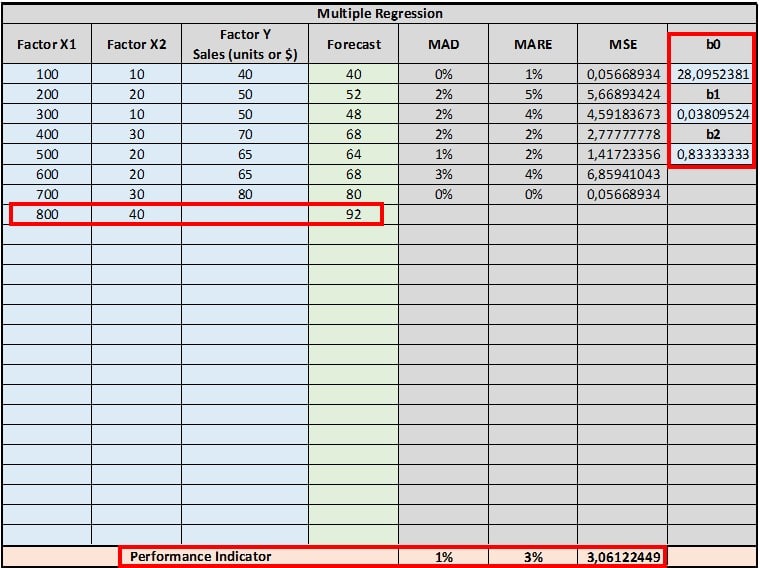
Step 5: Enter the data “b0”, “b1” and “b2” to generate the forecast calculations based on the multiple regression obtained. As you have new data, you can repeat the exercise to update the model (recalculate b0, b1, b2). Input data into X1 and X2 to generate forecasts.

 

 

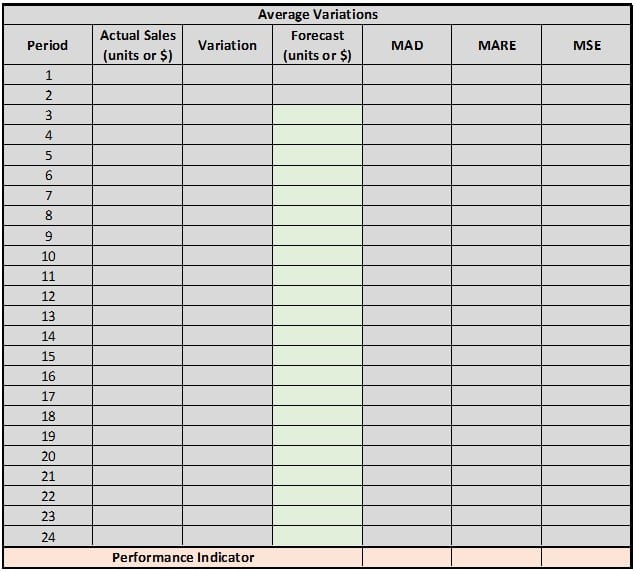
Average Variation

 

The method of mean variations is a method with generally low to medium precision. It is a simple and quick method to use. It requires little data to establish precision.

To use this method, the average change in sales is calculated to calculate the forecasts for the next periods. Here are the formulas used:

Variation =  (Actual sales period (i) – Actual sales period (i – 1)) / Actual sales period (i – 1)

Average increase = ∑ i to n (Variation / n)

Forecast for period (i+1) = Actual sale for period i * (100% + average increase)

 

Average Variation – Excel Tool

 

 

Double Moving Average (MMD)

 

The double moving average makes it possible to establish sales forecasts with average to good accuracy. This method is used for sales with an upward (or downward) trend, but without seasonality.

MMD consists of performing two moving averages to calculate a forecast, versus one with the simple moving average.

Mathematical formula :

Forecast I+i (T) = 2M_i – M_i^[2] +(i2 / n – 1)*(M_i – M_i^[2])

Where MI = Moving average at period I, MI[2] = Double moving average at period I, t = number of periods in the future, and n = number of periods used for simple and double moving average calculation.

 

Double Moving Average (MMD) – Excel Tool

 

 

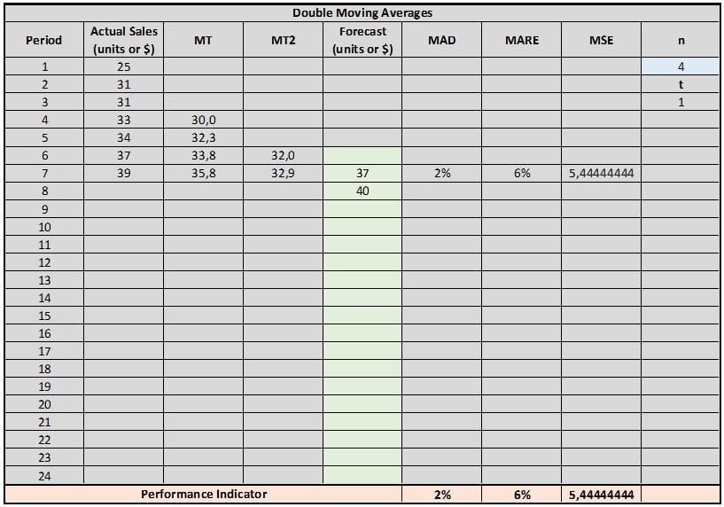
For this method, you can select an “n” equal to 3, 4, 5, or 6 to perform the moving average calculations. This makes it possible to obtain better precision and to make more or fewer forecasts with the same amount of data.

For example, with n = 6, it takes at least 11 data before obtaining 1 forecast. With an “n” = 3, we only need 5 data. However, the precision of the data varies between n = 3 and n =6. Depending on the sales, it is good to test different n to get the best possible accuracy.

 

Simple Exponential Smoothing With Trend

 

Single exponential smoothing is a model that often gives good results. When there is a trend in sales, a linear trend factor and a smoothing constant for the linear trend must be added.

The formulas used and automated in the Excel file for this technique are:

Yt = αV_t + (1- α)(P_t-1 + G_t-1)

With G_t = β(Y_t – Y_t-1)+(1-β)G_t-1

And P_t+1 = Y_T + G_T

Where Y_t = Estimated and smoothed sales at time t, V_t = Current sales at time t, G_t = smoothed linear trend factor, α = smoothing constant for random variation, β = smoothing constant for linear trend, and P_t = forecast for the period t.

Typically: 0.1 < α < 0.3 and 0.05 < β < 0.2

 

Simple Exponential Smoothing With Trend – Excel Tool

 

 

Enter your data into the table titled “Data” and select enter the α and β parameters in the blue boxes. Try different values ​​and stick with the one that best suits your situation. Rely on the performance indicators to make your choice!

 

Double Exponential Smoothing (DES)

 

The double exponential smoothing also makes it possible to obtain good forecasts. This is one of the models to watch because there is a good chance that it has the best performance indicators for you (i.e. the average deviations between forecasts and actual sales are low ).

Here is the procedure to perform LED. This method is already programmed in our free file, so you can skip this section if you wish. To interest them:

Let: X: Independent variable (period); Y: Dependent variable (sale)

To begin with, the initial estimates must be calculated using linear regression. To obtain an acceptable precision, it is recommended to use at least 8 data.

 

S₀ = P₀ – ((β/α) a) and S₀(2) = P₀  – (2 (β/α) * b)

 

Where (in the case where 8 data are used to do the linear regression) S0 = S8, S0(2) = S8(2), P0 = P8 = Forecast of the 8th period (calculate with the regression)

Once the initial estimates have been calculated, predictions can be made by double exponential smoothing.

 

P_0+t = P_8+t = (( 2 + (αt / β)) S₈ ) – (( 1 + (αt / β)) S₈(2))

S_0+t = α X_t + (1 – α)*S_0+t-1 and S_0+t(2) = α S0+t + (1 – α)*S_0+t-1(2)

 

Double Exponential Smoothing – Excel tool

 

 

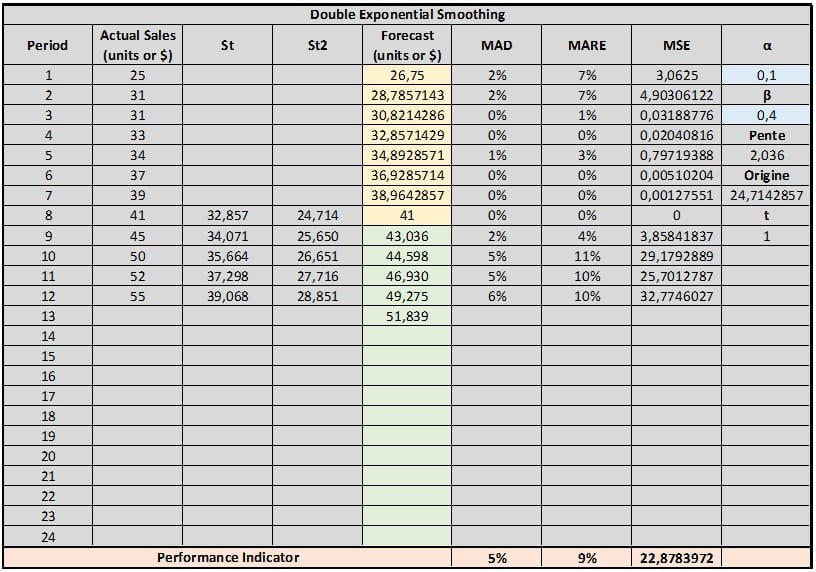
Experiment with values ​​of α and β to get the best model for your situation.

0 < α < 1 and 0 < β < 1

 

Forecasting Methods With Seasonality – Sales Forecasting

 

Seasonal Forecasts using Index

 

This first method of sales forecasting with seasonality does not use “seasonal adjustment” to perform the forecast calculations. It is rather with the help of the seasonal index that the forecasts are calculated. The method is simple and effective.

To demonstrate the principle, use the excel spreadsheet provided in the article.

 

Seasonal Forecasts using Index – Excel Tool

 

Step 1: Input your past sales data and calculate the sum of rows and columns

 

 

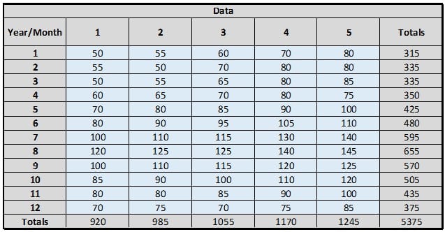
Step 2: Calculate the seasonal indices. To do this, divide the sum of a month by the total sales. For example, the index for January is calculated as follows:

 

315 / 5375 = 0.05860…

The total of the indices must be equal to 1.

 

 

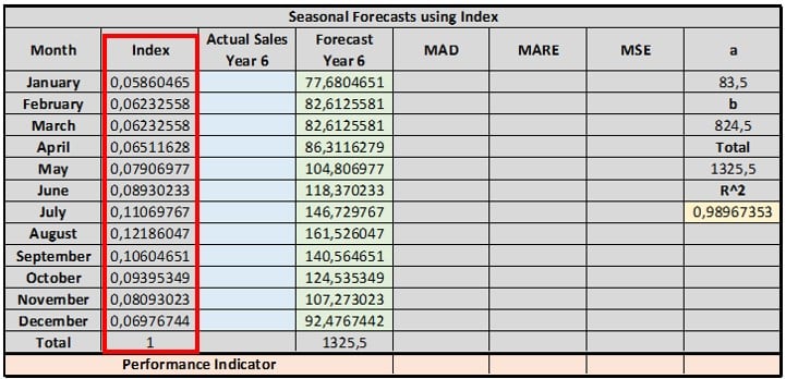
Step 3: Next, run the linear regression with the total year data.

 

 

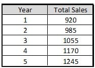
Y = aX + b = 83,5X + 824,5

 

 

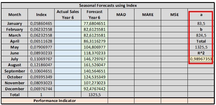
Step 4: Now, to make the predictions, use linear regression and seasonal indices.

 

For example, for January of the 6th year, the forecast will be:

Y = 83.5*6 + 824.5 = 1325.5

1325.5 * 0.05860465 = 77.68…

 

 

Other Methods For Seasonal Sales

 

There are other models for seasonal sales, including the Winters model, which offers good precision but is more complex than the other models and the seasonal adjustment methods.

For more information on these methods, contact us

 

 

Conclusion

 

Sales forecasts are a cornerstone for companies, because from them flow forecast budgets, optimal inventory management, etc. This can even make it easier to apply for funding.

In this article, a multitude of forecasting methods is presented and programmed in an Excel file. The methods are separated according to the company’s sales context (by level or stable, with the trend or with seasonality).

Finally, the various performance indicators allowing us to compare the methods and identify the best ones according to our situation are presented. In addition, these are also programmed in the Excel spreadsheet in order to compare the methods at a glance!